# Demo5 - Trace Parser
In this demo, you will learn how to model the `input` and `observations` events of a descrete event system (DES), and how to extract information from parsed counter example.
This demo shows a Node-Path-Node model: [NPNModel.xml](https://github.com/Jack0Chan/PyUPPAAL/tree/main/src/test_demos/NPNModel.xml), and the input node can accept input, and send it to output node via the path, where
1. The node has Refractory period, during which the node can do nothing.
2. The path has Conducting period, suggesting the time that a signal travel from one node to another.
3. The set of observable events is $\Sigma^o$=`[sigOut]`, the set of unobservable events is $\Sigma^{un}$=`[actPath, actNode]`, and the set of control events is $\Sigma^c$=`[sigIn]`.
 ## 1. Load the model, and get communication graph
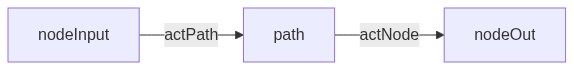
The communication graph shows the signal transfer relationship among the nodes and paths.
[](https://mermaid.live/edit#pako:eNpFjrsOwjAMRX-l8tz8QAYmFiRegg15sRKXVmqcKDgDqvrvmDIw-d6jI-suEHJk8PCsVMbueEMRAwcpTZ2joFfS0bldsYNStmL0bI7Rr3ppCj0krommaI8WlK5D0JETI3iLkQdqsyKgrKZS03x_SwCvtXEPrURS3k9kExL4geaX0ULyyPnfOU6a6-k3dtu8fgDk5EDN)
```python
import pyuppaal
from pyuppaal import UModel
pyuppaal.set_verifyta_path(r"C:\Users\10262\Documents\GitHub\cav2024\bin\uppaal64-4.1.26\bin-Windows\verifyta.exe")
umodel = UModel('NPNModel.xml').save_as('tmp_NPNModel.xml')
print(umodel.get_communication_graph())
```
```mermaid
graph TD
nodeInput--actPath-->path
path--actNode-->nodeOut
```
## 2. Construct the Input and Observation events
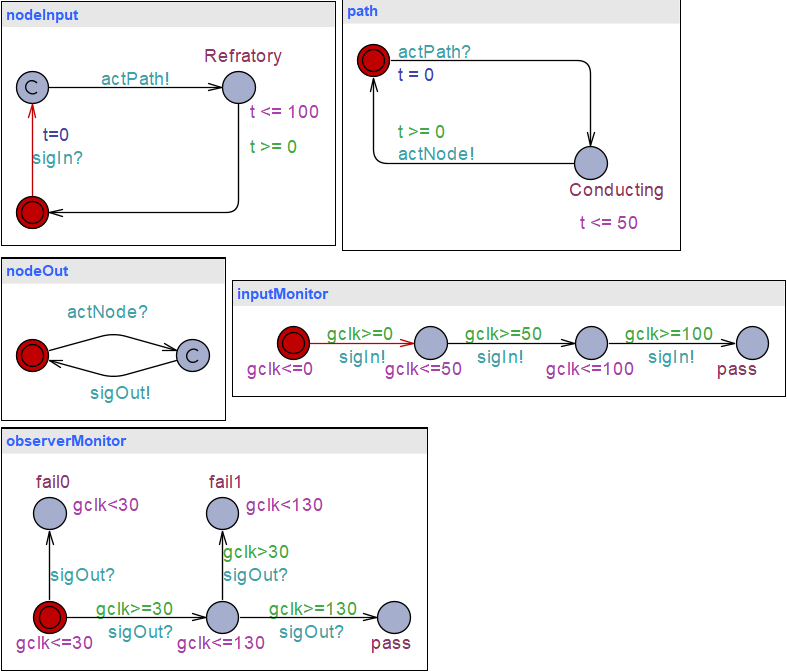
After sending `sigIn!` to `nodeInput` at time point `[0, 50, 100]`, we observed `sigOut!` from `nodeOut` at time point `[30, 130]`. `UModel.add_input_monitor()` and `UModel.add_observer_monitor()` will automatically add the constructed monitor into systems. After adding the `inputMonitor` and `observerMonitor` to current model, we get the following figure:
## 1. Load the model, and get communication graph
The communication graph shows the signal transfer relationship among the nodes and paths.
[](https://mermaid.live/edit#pako:eNpFjrsOwjAMRX-l8tz8QAYmFiRegg15sRKXVmqcKDgDqvrvmDIw-d6jI-suEHJk8PCsVMbueEMRAwcpTZ2joFfS0bldsYNStmL0bI7Rr3ppCj0krommaI8WlK5D0JETI3iLkQdqsyKgrKZS03x_SwCvtXEPrURS3k9kExL4geaX0ULyyPnfOU6a6-k3dtu8fgDk5EDN)
```python
import pyuppaal
from pyuppaal import UModel
pyuppaal.set_verifyta_path(r"C:\Users\10262\Documents\GitHub\cav2024\bin\uppaal64-4.1.26\bin-Windows\verifyta.exe")
umodel = UModel('NPNModel.xml').save_as('tmp_NPNModel.xml')
print(umodel.get_communication_graph())
```
```mermaid
graph TD
nodeInput--actPath-->path
path--actNode-->nodeOut
```
## 2. Construct the Input and Observation events
After sending `sigIn!` to `nodeInput` at time point `[0, 50, 100]`, we observed `sigOut!` from `nodeOut` at time point `[30, 130]`. `UModel.add_input_monitor()` and `UModel.add_observer_monitor()` will automatically add the constructed monitor into systems. After adding the `inputMonitor` and `observerMonitor` to current model, we get the following figure:
 ```python
# add input monitor
inputs = [('sigIn!', 'gclk>=0', 'gclk<=0'), ('sigIn!', 'gclk>=50', 'gclk<=50'), ('sigIn!', 'gclk>=100', 'gclk<=100')]
umodel.add_input_monitor(inputs=inputs, template_name='inputMonitor')
# add observer monitor
sigma_o = ['sigOut'] # observable events
obs = [('sigOut?', 'gclk>=30', 'gclk<=30'), ('sigOut?', 'gclk>=130', 'gclk<=130'), ]
umodel.add_observer_monitor(observations=obs, sigma_o=sigma_o, template_name='observerMonitor')
```
## 3. Sey queries and Verify the model
By querying `E<> observerMonitor.pass`, we can verify how the current model can simulate the current inputs and observations.
```python
# set queries
umodel.queries = ['E<> observerMonitor.pass']
# get SimTrace
st = umodel.easy_verify()
print(st)
```
State [0]: ['nodeInput._id2', 'path._id0', 'nodeOut._id5', 'inputMonitor._id7', 'observerMonitor._id11']
global_variables [0]: None
Clock_constraints [0]: [t(0) - gclk ≤ 0; t(0) - nodeInput.t ≤ 0; t(0) - path.t ≤ 0; gclk - nodeInput.t ≤ 0; nodeInput.t - path.t ≤ 0; path.t - t(0) ≤ 0; ]
transitions [0]: sigIn: inputMonitor -> nodeInput; inputMonitor._id7 -> inputMonitor._id8; nodeInput._id2 -> nodeInput._id4;
-----------------------------------
State [1]: ['nodeInput._id4', 'path._id0', 'nodeOut._id5', 'inputMonitor._id8', 'observerMonitor._id11']
global_variables [1]: None
Clock_constraints [1]: [t(0) - gclk ≤ 0; t(0) - nodeInput.t ≤ 0; t(0) - path.t ≤ 0; gclk - nodeInput.t ≤ 0; nodeInput.t - path.t ≤ 0; path.t - t(0) ≤ 0; ]
transitions [1]: actPath: nodeInput -> path; nodeInput._id4 -> nodeInput.Refratory; path._id0 -> path.Conducting;
-----------------------------------
State [2]: ['nodeInput.Refratory', 'path.Conducting', 'nodeOut._id5', 'inputMonitor._id8', 'observerMonitor._id11']
global_variables [2]: None
Clock_constraints [2]: [t(0) - gclk ≤ 0; t(0) - nodeInput.t ≤ 0; t(0) - path.t ≤ 0; gclk - t(0) ≤ 30; gclk - nodeInput.t ≤ 0; nodeInput.t - path.t ≤ 0; path.t - gclk ≤ 0; ]
transitions [2]: actNode: path -> nodeOut; path.Conducting -> path._id0; nodeOut._id5 -> nodeOut._id6;
-----------------------------------
State [3]: ['nodeInput.Refratory', 'path._id0', 'nodeOut._id6', 'inputMonitor._id8', 'observerMonitor._id11']
global_variables [3]: None
Clock_constraints [3]: [t(0) - gclk ≤ 0; t(0) - nodeInput.t ≤ 0; t(0) - path.t ≤ 0; gclk - t(0) ≤ 30; gclk - nodeInput.t ≤ 0; nodeInput.t - path.t ≤ 0; path.t - gclk ≤ 0; ]
transitions [3]: sigOut: nodeOut -> observerMonitor; nodeOut._id6 -> nodeOut._id5; observerMonitor._id11 -> observerMonitor._id12;
-----------------------------------
State [4]: ['nodeInput.Refratory', 'path._id0', 'nodeOut._id5', 'inputMonitor._id8', 'observerMonitor._id12']
global_variables [4]: None
Clock_constraints [4]: [t(0) - gclk ≤ -30; t(0) - nodeInput.t ≤ 0; t(0) - path.t ≤ 0; gclk - t(0) ≤ 50; gclk - nodeInput.t ≤ 0; nodeInput.t - path.t ≤ 0; path.t - gclk ≤ 0; ]
transitions [4]: sigIn: inputMonitor -> ; inputMonitor._id8 -> inputMonitor._id9;
-----------------------------------
State [5]: ['nodeInput.Refratory', 'path._id0', 'nodeOut._id5', 'inputMonitor._id9', 'observerMonitor._id12']
global_variables [5]: None
Clock_constraints [5]: [t(0) - gclk ≤ -50; t(0) - nodeInput.t ≤ 0; t(0) - path.t ≤ 0; gclk - t(0) ≤ 100; gclk - nodeInput.t ≤ 0; nodeInput.t - path.t ≤ 0; path.t - gclk ≤ 0; ]
transitions [5]: None: nodeInput -> nodeInput; nodeInput.Refratory -> nodeInput._id2;
-----------------------------------
State [6]: ['nodeInput._id2', 'path._id0', 'nodeOut._id5', 'inputMonitor._id9', 'observerMonitor._id12']
global_variables [6]: None
Clock_constraints [6]: [t(0) - gclk ≤ -50; t(0) - nodeInput.t ≤ 0; t(0) - path.t ≤ 0; gclk - t(0) ≤ 100; gclk - nodeInput.t ≤ 0; nodeInput.t - path.t ≤ 0; path.t - gclk ≤ 0; ]
transitions [6]: sigIn: inputMonitor -> nodeInput; inputMonitor._id9 -> inputMonitor.pass; nodeInput._id2 -> nodeInput._id4;
-----------------------------------
State [7]: ['nodeInput._id4', 'path._id0', 'nodeOut._id5', 'inputMonitor.pass', 'observerMonitor._id12']
global_variables [7]: None
Clock_constraints [7]: [t(0) - gclk ≤ -100; t(0) - nodeInput.t ≤ 0; t(0) - path.t ≤ 0; gclk - nodeInput.t ≤ 100; nodeInput.t - path.t ≤ -100; path.t - t(0) ≤ 100; ]
transitions [7]: actPath: nodeInput -> path; nodeInput._id4 -> nodeInput.Refratory; path._id0 -> path.Conducting;
-----------------------------------
State [8]: ['nodeInput.Refratory', 'path.Conducting', 'nodeOut._id5', 'inputMonitor.pass', 'observerMonitor._id12']
global_variables [8]: None
Clock_constraints [8]: [t(0) - gclk ≤ -100; t(0) - nodeInput.t ≤ 0; t(0) - path.t ≤ 0; gclk - t(0) ≤ 130; gclk - nodeInput.t ≤ 100; nodeInput.t - path.t ≤ 0; path.t - gclk ≤ -100; ]
transitions [8]: actNode: path -> nodeOut; path.Conducting -> path._id0; nodeOut._id5 -> nodeOut._id6;
-----------------------------------
State [9]: ['nodeInput.Refratory', 'path._id0', 'nodeOut._id6', 'inputMonitor.pass', 'observerMonitor._id12']
global_variables [9]: None
Clock_constraints [9]: [t(0) - gclk ≤ -100; t(0) - nodeInput.t ≤ 0; t(0) - path.t ≤ 0; gclk - t(0) ≤ 130; gclk - nodeInput.t ≤ 100; nodeInput.t - path.t ≤ 0; path.t - gclk ≤ -100; ]
transitions [9]: sigOut: nodeOut -> observerMonitor; nodeOut._id6 -> nodeOut._id5; observerMonitor._id12 -> observerMonitor.pass;
-----------------------------------
State [10]: ['nodeInput.Refratory', 'path._id0', 'nodeOut._id5', 'inputMonitor.pass', 'observerMonitor.pass']
global_variables [10]: None
Clock_constraints [10]: [t(0) - gclk ≤ -130; t(0) - nodeInput.t ≤ 0; t(0) - path.t ≤ 0; gclk - t(0) ≤ 200; gclk - nodeInput.t ≤ 100; nodeInput.t - path.t ≤ 0; path.t - gclk ≤ -100; ]
## 5. Analyze path conduction info
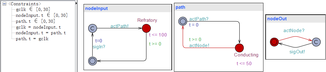
We can infer that `0<= path.t <=30` from `clock_constraints[3]`, meaning that the conduction period of the path may lie in `[0, 30]`.
```python
# add input monitor
inputs = [('sigIn!', 'gclk>=0', 'gclk<=0'), ('sigIn!', 'gclk>=50', 'gclk<=50'), ('sigIn!', 'gclk>=100', 'gclk<=100')]
umodel.add_input_monitor(inputs=inputs, template_name='inputMonitor')
# add observer monitor
sigma_o = ['sigOut'] # observable events
obs = [('sigOut?', 'gclk>=30', 'gclk<=30'), ('sigOut?', 'gclk>=130', 'gclk<=130'), ]
umodel.add_observer_monitor(observations=obs, sigma_o=sigma_o, template_name='observerMonitor')
```
## 3. Sey queries and Verify the model
By querying `E<> observerMonitor.pass`, we can verify how the current model can simulate the current inputs and observations.
```python
# set queries
umodel.queries = ['E<> observerMonitor.pass']
# get SimTrace
st = umodel.easy_verify()
print(st)
```
State [0]: ['nodeInput._id2', 'path._id0', 'nodeOut._id5', 'inputMonitor._id7', 'observerMonitor._id11']
global_variables [0]: None
Clock_constraints [0]: [t(0) - gclk ≤ 0; t(0) - nodeInput.t ≤ 0; t(0) - path.t ≤ 0; gclk - nodeInput.t ≤ 0; nodeInput.t - path.t ≤ 0; path.t - t(0) ≤ 0; ]
transitions [0]: sigIn: inputMonitor -> nodeInput; inputMonitor._id7 -> inputMonitor._id8; nodeInput._id2 -> nodeInput._id4;
-----------------------------------
State [1]: ['nodeInput._id4', 'path._id0', 'nodeOut._id5', 'inputMonitor._id8', 'observerMonitor._id11']
global_variables [1]: None
Clock_constraints [1]: [t(0) - gclk ≤ 0; t(0) - nodeInput.t ≤ 0; t(0) - path.t ≤ 0; gclk - nodeInput.t ≤ 0; nodeInput.t - path.t ≤ 0; path.t - t(0) ≤ 0; ]
transitions [1]: actPath: nodeInput -> path; nodeInput._id4 -> nodeInput.Refratory; path._id0 -> path.Conducting;
-----------------------------------
State [2]: ['nodeInput.Refratory', 'path.Conducting', 'nodeOut._id5', 'inputMonitor._id8', 'observerMonitor._id11']
global_variables [2]: None
Clock_constraints [2]: [t(0) - gclk ≤ 0; t(0) - nodeInput.t ≤ 0; t(0) - path.t ≤ 0; gclk - t(0) ≤ 30; gclk - nodeInput.t ≤ 0; nodeInput.t - path.t ≤ 0; path.t - gclk ≤ 0; ]
transitions [2]: actNode: path -> nodeOut; path.Conducting -> path._id0; nodeOut._id5 -> nodeOut._id6;
-----------------------------------
State [3]: ['nodeInput.Refratory', 'path._id0', 'nodeOut._id6', 'inputMonitor._id8', 'observerMonitor._id11']
global_variables [3]: None
Clock_constraints [3]: [t(0) - gclk ≤ 0; t(0) - nodeInput.t ≤ 0; t(0) - path.t ≤ 0; gclk - t(0) ≤ 30; gclk - nodeInput.t ≤ 0; nodeInput.t - path.t ≤ 0; path.t - gclk ≤ 0; ]
transitions [3]: sigOut: nodeOut -> observerMonitor; nodeOut._id6 -> nodeOut._id5; observerMonitor._id11 -> observerMonitor._id12;
-----------------------------------
State [4]: ['nodeInput.Refratory', 'path._id0', 'nodeOut._id5', 'inputMonitor._id8', 'observerMonitor._id12']
global_variables [4]: None
Clock_constraints [4]: [t(0) - gclk ≤ -30; t(0) - nodeInput.t ≤ 0; t(0) - path.t ≤ 0; gclk - t(0) ≤ 50; gclk - nodeInput.t ≤ 0; nodeInput.t - path.t ≤ 0; path.t - gclk ≤ 0; ]
transitions [4]: sigIn: inputMonitor -> ; inputMonitor._id8 -> inputMonitor._id9;
-----------------------------------
State [5]: ['nodeInput.Refratory', 'path._id0', 'nodeOut._id5', 'inputMonitor._id9', 'observerMonitor._id12']
global_variables [5]: None
Clock_constraints [5]: [t(0) - gclk ≤ -50; t(0) - nodeInput.t ≤ 0; t(0) - path.t ≤ 0; gclk - t(0) ≤ 100; gclk - nodeInput.t ≤ 0; nodeInput.t - path.t ≤ 0; path.t - gclk ≤ 0; ]
transitions [5]: None: nodeInput -> nodeInput; nodeInput.Refratory -> nodeInput._id2;
-----------------------------------
State [6]: ['nodeInput._id2', 'path._id0', 'nodeOut._id5', 'inputMonitor._id9', 'observerMonitor._id12']
global_variables [6]: None
Clock_constraints [6]: [t(0) - gclk ≤ -50; t(0) - nodeInput.t ≤ 0; t(0) - path.t ≤ 0; gclk - t(0) ≤ 100; gclk - nodeInput.t ≤ 0; nodeInput.t - path.t ≤ 0; path.t - gclk ≤ 0; ]
transitions [6]: sigIn: inputMonitor -> nodeInput; inputMonitor._id9 -> inputMonitor.pass; nodeInput._id2 -> nodeInput._id4;
-----------------------------------
State [7]: ['nodeInput._id4', 'path._id0', 'nodeOut._id5', 'inputMonitor.pass', 'observerMonitor._id12']
global_variables [7]: None
Clock_constraints [7]: [t(0) - gclk ≤ -100; t(0) - nodeInput.t ≤ 0; t(0) - path.t ≤ 0; gclk - nodeInput.t ≤ 100; nodeInput.t - path.t ≤ -100; path.t - t(0) ≤ 100; ]
transitions [7]: actPath: nodeInput -> path; nodeInput._id4 -> nodeInput.Refratory; path._id0 -> path.Conducting;
-----------------------------------
State [8]: ['nodeInput.Refratory', 'path.Conducting', 'nodeOut._id5', 'inputMonitor.pass', 'observerMonitor._id12']
global_variables [8]: None
Clock_constraints [8]: [t(0) - gclk ≤ -100; t(0) - nodeInput.t ≤ 0; t(0) - path.t ≤ 0; gclk - t(0) ≤ 130; gclk - nodeInput.t ≤ 100; nodeInput.t - path.t ≤ 0; path.t - gclk ≤ -100; ]
transitions [8]: actNode: path -> nodeOut; path.Conducting -> path._id0; nodeOut._id5 -> nodeOut._id6;
-----------------------------------
State [9]: ['nodeInput.Refratory', 'path._id0', 'nodeOut._id6', 'inputMonitor.pass', 'observerMonitor._id12']
global_variables [9]: None
Clock_constraints [9]: [t(0) - gclk ≤ -100; t(0) - nodeInput.t ≤ 0; t(0) - path.t ≤ 0; gclk - t(0) ≤ 130; gclk - nodeInput.t ≤ 100; nodeInput.t - path.t ≤ 0; path.t - gclk ≤ -100; ]
transitions [9]: sigOut: nodeOut -> observerMonitor; nodeOut._id6 -> nodeOut._id5; observerMonitor._id12 -> observerMonitor.pass;
-----------------------------------
State [10]: ['nodeInput.Refratory', 'path._id0', 'nodeOut._id5', 'inputMonitor.pass', 'observerMonitor.pass']
global_variables [10]: None
Clock_constraints [10]: [t(0) - gclk ≤ -130; t(0) - nodeInput.t ≤ 0; t(0) - path.t ≤ 0; gclk - t(0) ≤ 200; gclk - nodeInput.t ≤ 100; nodeInput.t - path.t ≤ 0; path.t - gclk ≤ -100; ]
## 5. Analyze path conduction info
We can infer that `0<= path.t <=30` from `clock_constraints[3]`, meaning that the conduction period of the path may lie in `[0, 30]`.
 ```python
print(f"states: {st.states[3]}")
print(f"clock constraints: {st.clock_constraints[3]}")
print(f"transitions: {st.transitions[3]}")
print("\n======== Analysis ========")
print("We can infer that `0<=path.t<=30` from the following clock constraints:")
for clk_zone in [st.clock_constraints[3][2], st.clock_constraints[3][3], st.clock_constraints[3][-1]]:
print(clk_zone)
```
states: ['nodeInput.Refratory', 'path._id0', 'nodeOut._id6', 'inputMonitor._id8', 'observerMonitor._id11']
clock constraints: [t(0) - gclk ≤ 0; t(0) - nodeInput.t ≤ 0; t(0) - path.t ≤ 0; gclk - t(0) ≤ 30; gclk - nodeInput.t ≤ 0; nodeInput.t - path.t ≤ 0; path.t - gclk ≤ 0; ]
transitions: sigOut: nodeOut -> observerMonitor; nodeOut._id6 -> nodeOut._id5; observerMonitor._id11 -> observerMonitor._id12;
======== Analysis ========
We can infer that `0<=path.t<=30` from the following clock constraints:
[t(0) - path.t ≤ 0]
[gclk - t(0) ≤ 30]
[path.t - gclk ≤ 0]
## 4. Analyze node refractory info
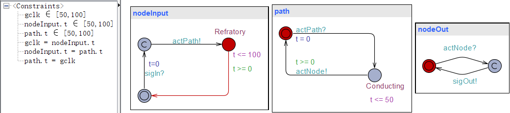
We can infer that `50<= nodeInput.t <=100` from `clock_constraints[5]`, meaning that the refractory period of the input node may lie in `[50, 100]`.
```python
print(f"states: {st.states[3]}")
print(f"clock constraints: {st.clock_constraints[3]}")
print(f"transitions: {st.transitions[3]}")
print("\n======== Analysis ========")
print("We can infer that `0<=path.t<=30` from the following clock constraints:")
for clk_zone in [st.clock_constraints[3][2], st.clock_constraints[3][3], st.clock_constraints[3][-1]]:
print(clk_zone)
```
states: ['nodeInput.Refratory', 'path._id0', 'nodeOut._id6', 'inputMonitor._id8', 'observerMonitor._id11']
clock constraints: [t(0) - gclk ≤ 0; t(0) - nodeInput.t ≤ 0; t(0) - path.t ≤ 0; gclk - t(0) ≤ 30; gclk - nodeInput.t ≤ 0; nodeInput.t - path.t ≤ 0; path.t - gclk ≤ 0; ]
transitions: sigOut: nodeOut -> observerMonitor; nodeOut._id6 -> nodeOut._id5; observerMonitor._id11 -> observerMonitor._id12;
======== Analysis ========
We can infer that `0<=path.t<=30` from the following clock constraints:
[t(0) - path.t ≤ 0]
[gclk - t(0) ≤ 30]
[path.t - gclk ≤ 0]
## 4. Analyze node refractory info
We can infer that `50<= nodeInput.t <=100` from `clock_constraints[5]`, meaning that the refractory period of the input node may lie in `[50, 100]`.
 ```python
print(f"states: {st.states[5]}")
print(f"clock constraints: {st.clock_constraints[5]}")
print(f"transitions: {st.transitions[5]}")
print("\n======== Analysis ========")
print("We can infer that `50<=nodeInput.t<=100` from the following clock constraints:")
for clk_zone in [st.clock_constraints[5][0], st.clock_constraints[5][3], st.clock_constraints[3][4], st.clock_constraints[3][5]]:
print(clk_zone)
```
states: ['nodeInput.Refratory', 'path._id0', 'nodeOut._id5', 'inputMonitor._id9', 'observerMonitor._id12']
clock constraints: [t(0) - gclk ≤ -50; t(0) - nodeInput.t ≤ 0; t(0) - path.t ≤ 0; gclk - t(0) ≤ 100; gclk - nodeInput.t ≤ 0; nodeInput.t - path.t ≤ 0; path.t - gclk ≤ 0; ]
transitions: None: nodeInput -> nodeInput; nodeInput.Refratory -> nodeInput._id2;
======== Analysis ========
We can infer that `50<=nodeInput.t<=100` from the following clock constraints:
[t(0) - gclk ≤ -50]
[gclk - t(0) ≤ 100]
[gclk - nodeInput.t ≤ 0]
[nodeInput.t - path.t ≤ 0]
```python
print(f"states: {st.states[5]}")
print(f"clock constraints: {st.clock_constraints[5]}")
print(f"transitions: {st.transitions[5]}")
print("\n======== Analysis ========")
print("We can infer that `50<=nodeInput.t<=100` from the following clock constraints:")
for clk_zone in [st.clock_constraints[5][0], st.clock_constraints[5][3], st.clock_constraints[3][4], st.clock_constraints[3][5]]:
print(clk_zone)
```
states: ['nodeInput.Refratory', 'path._id0', 'nodeOut._id5', 'inputMonitor._id9', 'observerMonitor._id12']
clock constraints: [t(0) - gclk ≤ -50; t(0) - nodeInput.t ≤ 0; t(0) - path.t ≤ 0; gclk - t(0) ≤ 100; gclk - nodeInput.t ≤ 0; nodeInput.t - path.t ≤ 0; path.t - gclk ≤ 0; ]
transitions: None: nodeInput -> nodeInput; nodeInput.Refratory -> nodeInput._id2;
======== Analysis ========
We can infer that `50<=nodeInput.t<=100` from the following clock constraints:
[t(0) - gclk ≤ -50]
[gclk - t(0) ≤ 100]
[gclk - nodeInput.t ≤ 0]
[nodeInput.t - path.t ≤ 0]